Velocity-based validation

After an analysis, some vectors will be wrong — spurious correlations, noise, or outliers. This panel finds and removes them using statistical filters, a velocity-space limit you draw yourself, and manual clicking, then optionally fills the gaps by interpolation.

Open via Validation → Velocity based validation (Ctrl+V).

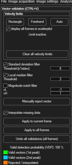
A sensible order Try Velocity limits first to catch the big, obvious outliers, then enable the Standard deviation and Local median filters. Reach for image-based validation only if problems remain after that.

PIVlab Vector validation panel with real analysis results — The **Vector validation** panel, showing real results (VDP 100% here since the demo data is clean).

Velocity limits

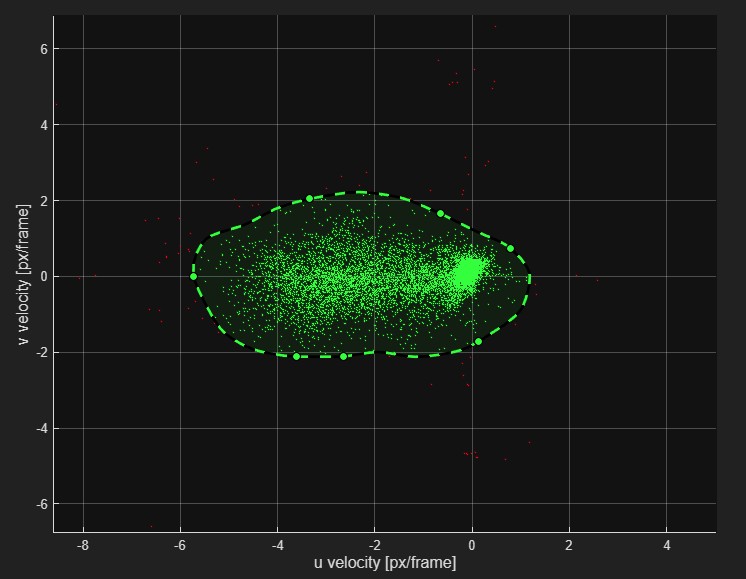
Click Rectangle, Freehand or Auto to open a scatter plot of every vector's u vs. v component (not its position in the image — its value in velocity space). Valid vectors cluster together; outliers sit far from the cluster.

Button	How you define the limit
Rectangle	Draw a rectangular window around the allowed velocities.
Freehand	Freely draw any shape around the allowed velocities.
Auto	PIVlab automatically draws a shape around the main cluster.

Any vector falling outside the shape you defined is treated as invalid. The display all frames in scatterplot checkbox (on by default) pools every frame's vectors into one scatter plot, which usually gives a clearer picture of the true cluster than a single frame would. Click Clear all velocity limits to remove the limit and start over.

Velocity scatter plot of u vs. v, with a green dashed shape drawn around the main cluster; outliers outside it are red — The velocity scatter plot with an Auto limit (green dashed). Green points are inside the limit and kept; red points fall outside and are rejected as outliers.

Statistical filters

Filter	Parameter	What it does
Standard deviation filter	Threshold [n × stdev] (default 4.7)	Removes vectors outside the mean velocity ± n times the standard deviation.
Local median filter	Threshold (default 3)	The normalized local median test (Westerweel & Scarano, 2005) — compares each vector to its immediate neighbours rather than the whole field, catching localized outliers a global filter would miss.
Magnitude notch filter	vL / vH (default −1 / 1)	Discards velocities that fall inside the range from vL to vH — the opposite of the other filters, useful for rejecting a specific unwanted velocity band (e.g. near-zero noise).

Both the standard-deviation and local-median filters are enabled by default; the notch filter is off by default.

Manually rejecting vectors

Click Manually reject vector, then click the base of any vector in the plot to discard it individually — useful for the odd bad vector the automatic filters don't catch.

Filling the gaps

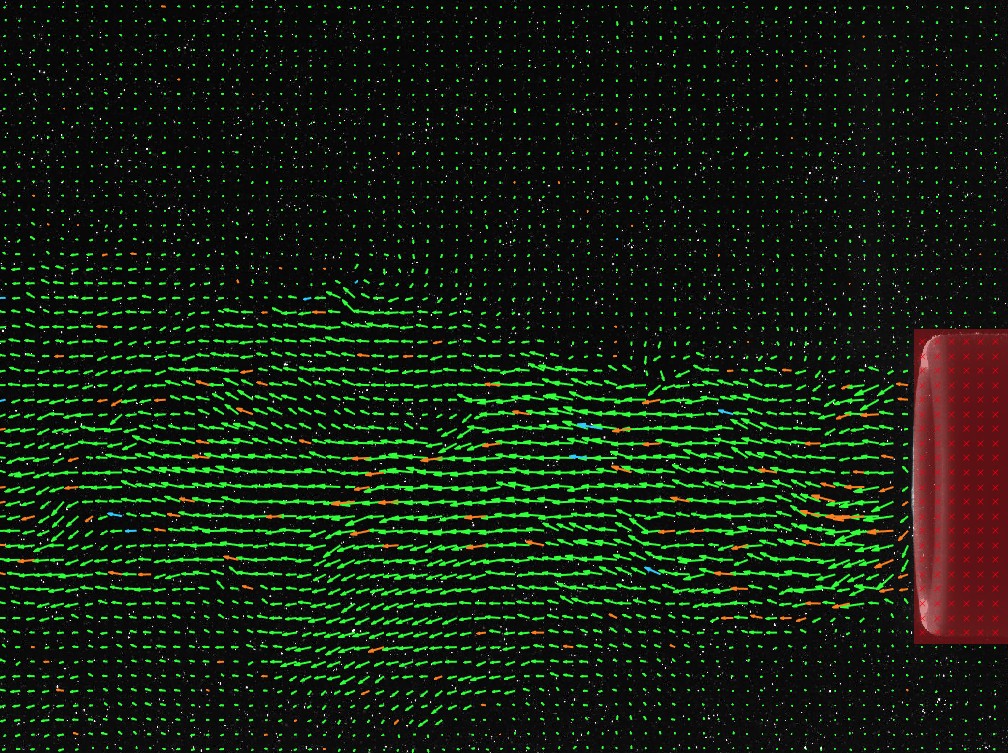
Interpolate missing data (on by default) fills rejected/missing vectors by interpolating from their neighbours. Interpolated vectors are drawn in orange in the plot, so you can always tell real data from filled-in data.

Interpolated vectors are not measurements An orange vector is a filled-in estimate, not something PIVlab actually measured. A few scattered interpolated vectors are normal and fine. A lot of them is a warning sign — it usually means poor image quality or unsuitable settings somewhere upstream, not something to overlook just because the vector field looks visually complete. See Troubleshooting by symptom if you're seeing large interpolated regions.

Tuning strategy: isolate, then combine

With several filters available, it's easy to end up with a combination that "looks right" without actually knowing which filter is doing what. A more reliable approach:

Tune one filter at a time — disable the others while you do.
Check that this filter, on its own, only removes vectors that are actually bad. If it's also eating good vectors, its threshold is too aggressive.
Step through a few different frames while checking — a threshold tuned on one frame doesn't always hold up across the rest of your dataset.
Once each filter is individually tuned, enable them all together.

A good sign If the filters still work well once combined, that's a strong indication they're catching almost all the erroneous vectors in your data.

Applying and undoing

Set up your limits and filters (see Tuning strategy above).
Click Apply to current frame to test on one frame, or Apply to all frames to validate the whole session.
Click Undo all validations (all frames) to remove every filter's effect and start over.

Reading the result

After validating, the panel shows the Valid detection probability (VDP) — the percentage of vectors that passed validation unmodified. As a rule of thumb, a VDP above 90% in the area you actually care about is fine — don't worry about a lower overall VDP if it's being dragged down by a region outside your area of interest (e.g. a masked object or the image border). The vector plot uses a color code:

Color	Meaning
Green	Valid vectors (1st correlation peak)
Cyan	Valid vectors (2nd correlation peak)
Orange	Rejected / interpolated

Vector field colour-coded by type: mostly green valid vectors, a few orange rejected/interpolated ones and cyan second-peak vectors, with the masked object shown in red — The validated vector field colour-coded by type — green (valid), orange (rejected / interpolated) and cyan (2nd peak). The red region is a mask.

Colors are configurable These three colors can be changed in Modify plot appearance — the swatches in this panel update to match whatever you choose there.

Also see image-based validation Image-based validation rejects vectors using the underlying image quality (contrast, glare, correlation) instead of the velocity value — independent of these filters, and worth combining with them.