Deriving spatial parameters / modifying data

Beyond raw velocity vectors, PIVlab can compute and display a range of derived flow quantities, smooth your data, and subtract a background flow — all without re-running the PIV analysis.

Open via Plot → Spatial: Derive parameters / modify data (Ctrl+D).

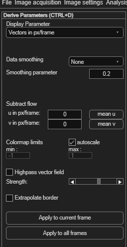
PIVlab Derive Parameters panel — The **Derive Parameters** panel.

Choosing what to display

The Display Parameter dropdown selects what's shown as a colour-coded overlay on the vector plot:

Parameter	Notes
Vectors	Raw velocity vectors (the default).
Vorticity	Local rotation of the flow.
Magnitude	Speed, regardless of direction.
u component / v component	Horizontal / vertical velocity only.
Divergence	Net outflow/inflow at each point.
Q criterion	A common vortex-identification measure.
Shear rate	Magnitude of the rate-of-strain tensor.
Simple strain rate	A simpler strain-rate estimate.
Line integral convolution (LIC)	A texture-based visualization of flow direction. Reveals streak-like structure; see the resolution slider below.
Vector direction	Angle in degrees.
Correlation coefficient	Quality of the underlying correlation.
Uncertainty	Only available if you enabled uncertainty estimation in PIV settings.

Units shown in the dropdown adapt automatically: pixels/frame if uncalibrated, meters/frame if calibrated with a zero time step (displacements only), or meters/second once fully calibrated.

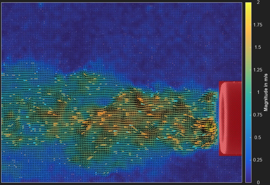
Velocity magnitude shown as a colour overlay on the vector field, with a colour bar labelled Magnitude in m/s and the masked object in red — Velocity Magnitude displayed as a colour overlay with the vectors on top and a labelled colour bar. The colour map, opacity and colour bar are all configurable in Modify plot appearance.

When Line integral convolution (LIC) is selected, a LIC resolution slider appears — higher values look more detailed but take longer to compute.

How each parameter is computed

This section gives the exact definition behind every entry in the dropdown, so you can check, cite or reproduce the numbers PIVlab reports.

Throughout, u and v are the velocity components along x and y, and u₀ / v₀ are the constant offsets you can enter under Subtract flow. The notation ∂u/∂y means “the rate at which u changes as you move in the y direction”.

Derivatives are taken on the calibrated grid Before any derivative is computed, the measurement grid is converted from pixels to metres and the velocities to m/s (using your spatial calibration). That is why the gradient-based quantities below come out per second rather than per frame. Without a calibration the same equations apply, but in px and frames — which is exactly what the units in the dropdown tell you.

Velocity-based quantities

These need no derivatives — they are computed point by point from the vectors themselves, and they are the only ones affected by Subtract flow.

Magnitude — the speed, i.e. the length of the velocity vector:

|V| = √( (u − u₀)² + (v − v₀)² )

u component and v component are simply u − u₀ and v − v₀.

Vector direction — the angle of each vector, via atan2d, reported between −180° and +180°:

θ = atan2(v − v₀, u − u₀)

With PIVlab's default axis settings (x increases towards the right, y increases towards the bottom — the usual image convention) the angles line up like this:

Angle	Direction on screen
0°	→ to the right
+90°	↓ downwards
+180° / −180°	← to the left
−90°	↑ upwards

So 0° points right, and angles increase clockwise as you see them on screen. If you set y increases towards the top in the calibration panel, the sign of v flips and angles then increase counter-clockwise instead, with +90° pointing up.

Gradient-based quantities

These are all built from the four spatial derivatives of the velocity field (∂u/∂x, ∂u/∂y, ∂v/∂x, ∂v/∂y), evaluated with MATLAB's gradient (central differences inside the field, one-sided at the edges).

Subtract flow does not change any of these Subtracting a constant velocity shifts every vector by the same amount, and a constant has no gradient — so vorticity, divergence, shear rate, strain rate and the Q criterion are deliberately computed from the unshifted field. Only the velocity-based quantities above respond to it.

Vorticity — the local rate of rotation of the fluid, computed with MATLAB's curl:

ω = ∂v/∂x − ∂u/∂y

PIVlab negates MATLAB's result, which sounds odd but is exactly what you want: image coordinates run with y pointing down, and the sign flip cancels that out. The result is the conventional definition above, so positive vorticity means counter-clockwise rotation as it appears on your screen.

Divergence — the net rate at which fluid flows out of each point, via MATLAB's divergence:

∇·V = ∂u/∂x + ∂v/∂y

For an incompressible flow measured in-plane this should be near zero, so a divergence map doubles as a rough sanity check on your data (or a sign of out-of-plane motion).

Shear rate — the magnitude of the rate-of-strain tensor. Writing its three independent components as

D_xx = ∂u/∂x
D_yy = ∂v/∂y
D_xy = ½ ( ∂u/∂y + ∂v/∂x )

the reported value is

‖D‖ = √( 2 ( D_xx² + D_yy² + 2 D_xy² ) )

This definition changed in PIVlab 3.10 Before version 3.10, Shear rate returned the simpler ∂v/∂x + ∂u/∂y. If you are comparing against results produced by an older PIVlab version, the two are not interchangeable.

Simple strain rate — the difference between the two normal strain rates:

∂u/∂x − ∂v/∂y

“Simple strain rate” is not the full strain rate Despite the name, this is a single combination of two derivatives, not the magnitude of the strain-rate tensor. If you want the complete measure, use Shear rate above.

Q criterion — a standard vortex-identification measure that compares rotation against strain. It is defined from the rotation tensor Ω and the strain-rate tensor S as ½(‖Ω‖² − ‖S‖²), where ‖·‖² means “the sum of the squares of all components”. Written out for a 2D field:

Q = ½ [ ½ (∂v/∂x − ∂u/∂y)² − (∂u/∂x)² − (∂v/∂y)² − 2 ( ½ (∂u/∂y + ∂v/∂x) )² ]

Positive Q marks regions where rotation dominates over strain — the usual criterion for identifying a vortex core. This calculation assumes an evenly spaced measurement grid, which is what a standard PIV analysis produces.

Quantities carried over from the analysis

The last three are not calculated on this panel at all — they are produced during the PIV analysis itself and simply displayed here.

Correlation coefficient — for each interrogation window, the Pearson correlation between the two image patches:

R = Σ(a·b) ⁄ √( Σa² · Σb² )

where a and b are the two interrogation windows with their mean brightness subtracted.

Crucially, this is evaluated on the final pass, after the windows have been deformed by the displacement measured up to that point. So it does not tell you how similar the two raw images were — it tells you how well the two windows match once they have been shifted and deformed by the vector PIVlab found. A value near 1 means the measured displacement really does explain the particle pattern; a low value flags a suspect vector. Masked windows are reported as 0. You can filter on exactly this quantity in image-based validation.

Uncertainty — an estimate of the error on each vector, in the same units as the velocity. PIVlab uses the particle-image disparity method: after both images are fully deformed by the measured displacement, any residual mismatch between individual particle pairs is measured, and the RMS spread of those mismatches within each interrogation window becomes the uncertainty (the x and y parts are combined as √(e_x² + e_y²)). The implementation follows:

Sciacchitano A, Wieneke B and Scarano F (2013), PIV uncertainty quantification by image matching, Meas. Sci. Technol. 24 045302, doi:10.1088/0957-0233/24/4/045302 — adapted from the MATLAB package by Dr. A. Sciacchitano (TU Delft).

A high uncertainty can mean two very different things Either the vector really is unreliable — too few particles, noisy images, or particles moving out of the light sheet — or the vector is correct but the flow varies strongly within the interrogation window, as happens at shear layers, sharp gradients and vortex cores. In the second case it is a spatial-resolution warning rather than a measurement error, telling you a smaller interrogation area would resolve more.

This map only exists if Compute uncertainty was enabled in PIV settings before the analysis ran; otherwise PIVlab tells you there is no uncertainty data for the frame.

Line integral convolution (LIC) has no closed-form equation. It smears a random noise image along the local flow direction, which makes streak-like patterns emerge that follow the vector field — a texture, not a measured quantity, so it carries no units and is always drawn with a gray colormap. PIVlab runs the process twice, feeding each result back in as the noise input for the next round. The technique was introduced by Cabral & Leedom (Imaging vector fields using line integral convolution, SIGGRAPH '93); PIVlab's implementation comes from the Matlab VFV Toolbox 1.0, by courtesy of Nima Bigdely Shamlo, Computational Science Research Center, San Diego State University.

Data smoothing

Mode	Effect
None	No smoothing (default).
2D	Spatial smoothing within each frame, using Damien Garcia's `smoothn`. Controlled by Smoothing parameter (default 0.2; larger = smoother, typical range 0.1–1).
time (moving average)	A moving average across neighbouring frames. Temporal window (± frames) sets how many frames on each side to include, combined with more weight given to closer frames.
2D + time	Both, spatial smoothing first, then temporal.

Smoothing happens before the derivatives Whatever you select here is applied to the velocity field first, and the derived parameters are then computed from the smoothed result. This matters because differentiating amplifies noise: a vorticity or Q-criterion map from an unsmoothed field is often far speckier than the underlying flow really is. PIVlab likewise uses your validated vectors when validation has been run, and can fill in rejected vectors first if interpolate missing data is enabled.

Subtracting a background flow

To reveal flow structure relative to a moving reference frame (e.g. removing a convection velocity), subtract a constant velocity from every vector:

Type a value directly into u: or v: to subtract a fixed velocity.
Or click mean u / mean v to subtract the field's own average automatically.

A separate, temporary highpass is also available Highpass vector field (with a Strength slider) removes a non-uniform background flow for display purposes — unlike the subtract-flow fields above, this modified data is not saved, only shown.

Colormap and display

Control	Effect
autoscale	Stretches the colour map to each frame's own min/max. Turn this off when rendering a video, so the color scale stays consistent across frames.
min / max	Manual colour-map bounds, editable once autoscale is off.
Extrapolate border	Fills the border region using spring inpainting instead of the mean value — slower, but smoother-looking.

Applying

Click Apply to current frame to preview on the current frame, or Apply to all frames to compute the selected parameter and settings across the whole session.

Combining data across frames instead? See Deriving temporal parameters — mean, sum, standard deviation and turbulent kinetic energy across a whole time-resolved sequence.