How stereo-PIV works: illustrated step by step
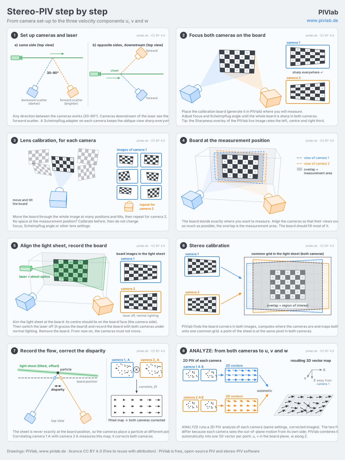
Stereo-PIV (stereoscopic particle image velocimetry, also called 2D3C) measures all three velocity components in a light sheet: u and v in the plane of the sheet and w through it. It needs two cameras that look at the sheet from different directions. This page explains the whole procedure in eight drawings, from setting up the cameras to the 3D vector map. The procedure is general; for the details in PIVlab, see the manual pages Stereo-PIV: set-up and recording (steps 1–5 and the recording) and Stereo-PIV analysis (steps 6–8).
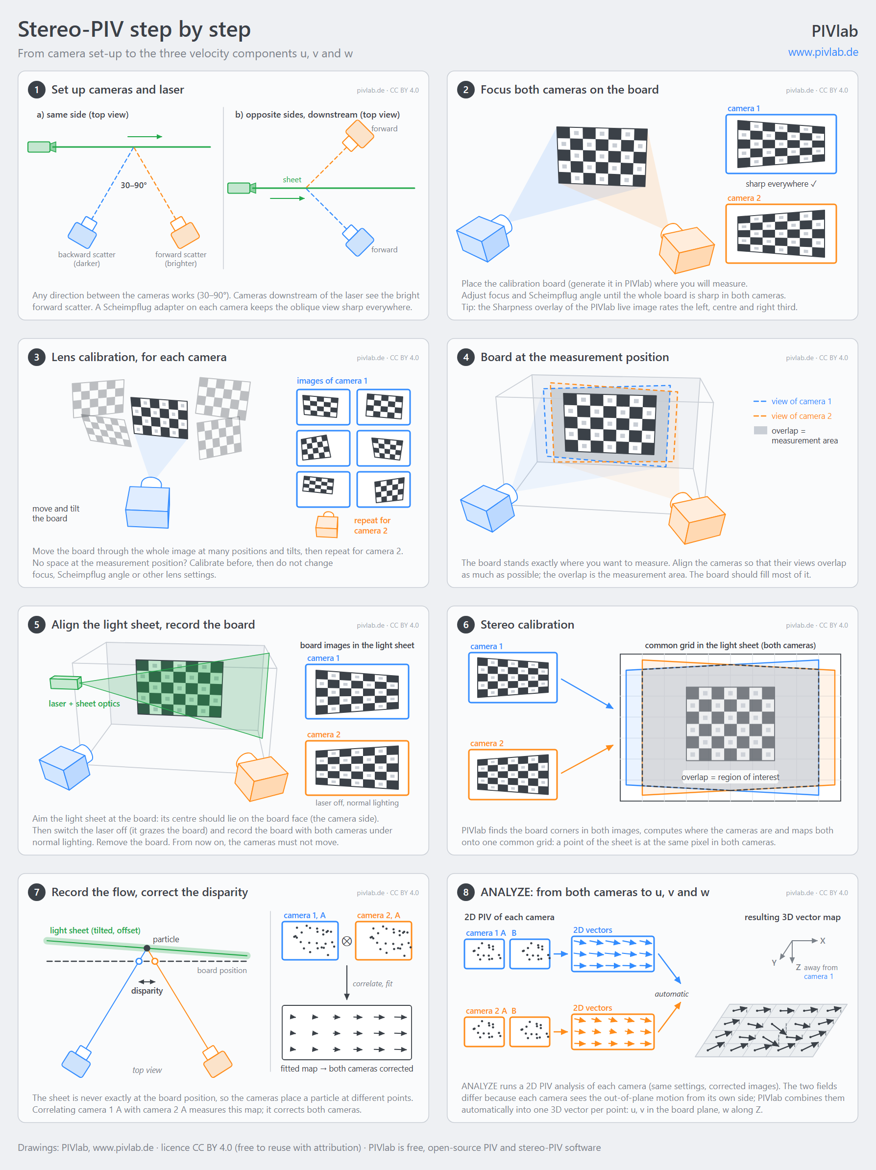
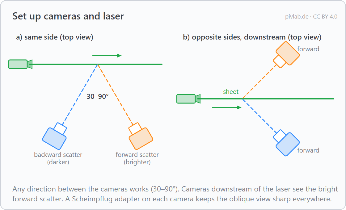
1. Set up cameras and laser
Both cameras look at the same part of the light sheet, but from different directions. The out-of-plane velocity w follows from the difference between their two views, so the angle between the lines of sight matters: 30° to 90° is good, a small angle makes w noisy. Two cameras that look at each other along one line can not measure w.
The particles are much brighter in forward scatter, i.e. for a camera downstream of the laser, than in backward scatter. With both cameras on the same side of the sheet, one of them usually sees backward scatter. Placing the cameras on opposite sides of the sheet, both downstream, gives both cameras forward scatter; the camera behind the board then needs a transparent board (or one printed mirrored on its back).
Because each camera looks at the sheet at an angle, a normal lens can not keep the whole sheet in focus. A Scheimpflug adapter tilts the lens against the sensor, so that the oblique plane is sharp everywhere.
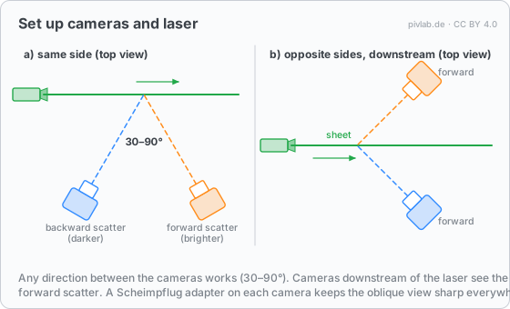
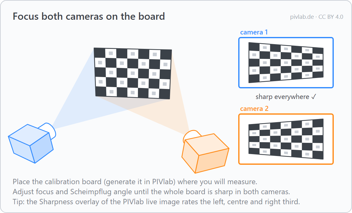
2. Focus both cameras on the board
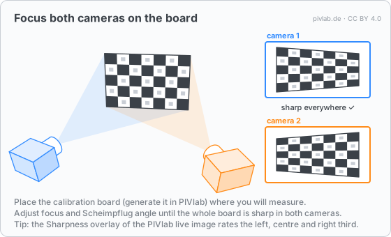
Place the calibration board where you will measure and focus both cameras on it. With Scheimpflug adapters, adjust focus and tilt until the whole board is sharp in both images. In PIVlab, the board is generated by the program (ChArUco board with a QR code that holds its dimensions), and the Sharpness overlay of the live image rates the focus in the left, centre and right third of the image.
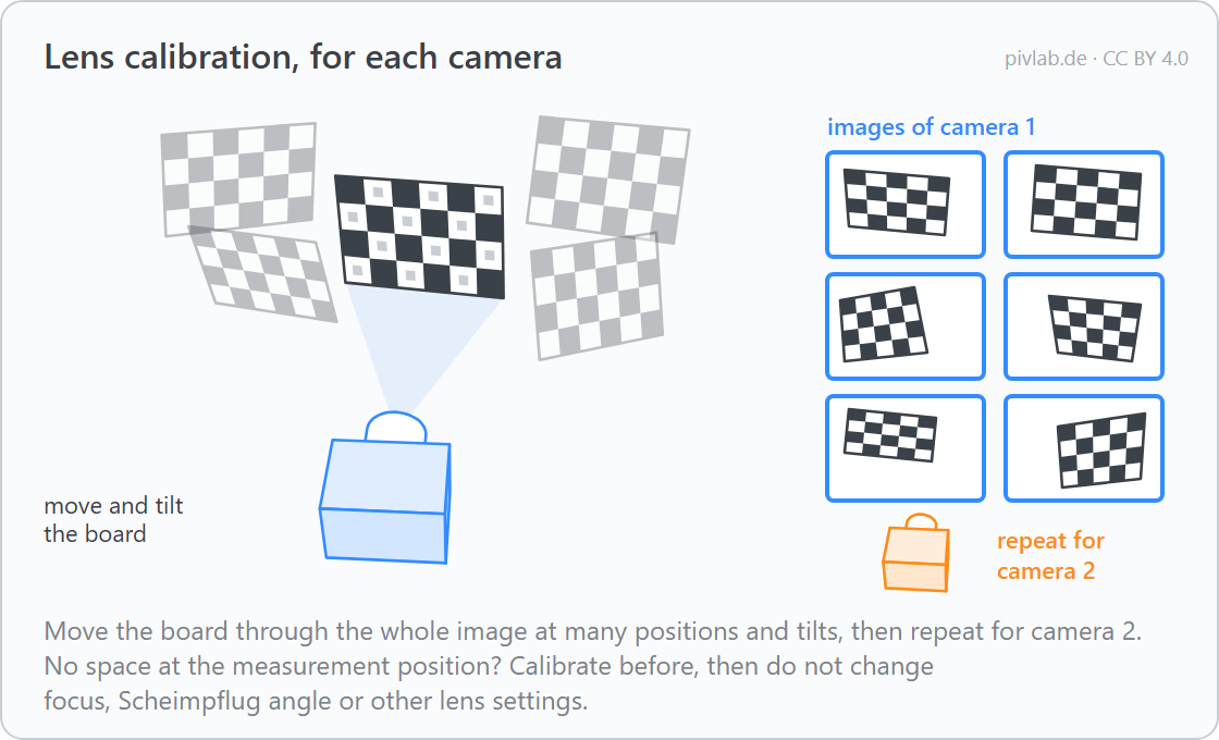
3. Lens calibration, for each camera
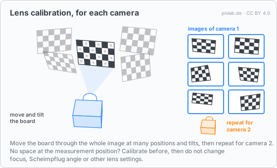
Each camera gets its own lens calibration: move the board through the whole image, at many positions and tilts, and record an image each time. From these images the lens distortion (and, with a Scheimpflug adapter, the tilt of the sensor) is computed. Repeat this for the second camera.
The lens calibration is only valid for these lens settings. If there is no space at the measurement position, it can be done beforehand; afterwards focus, Scheimpflug angle and the other lens settings must not change. The cameras themselves may still be moved.
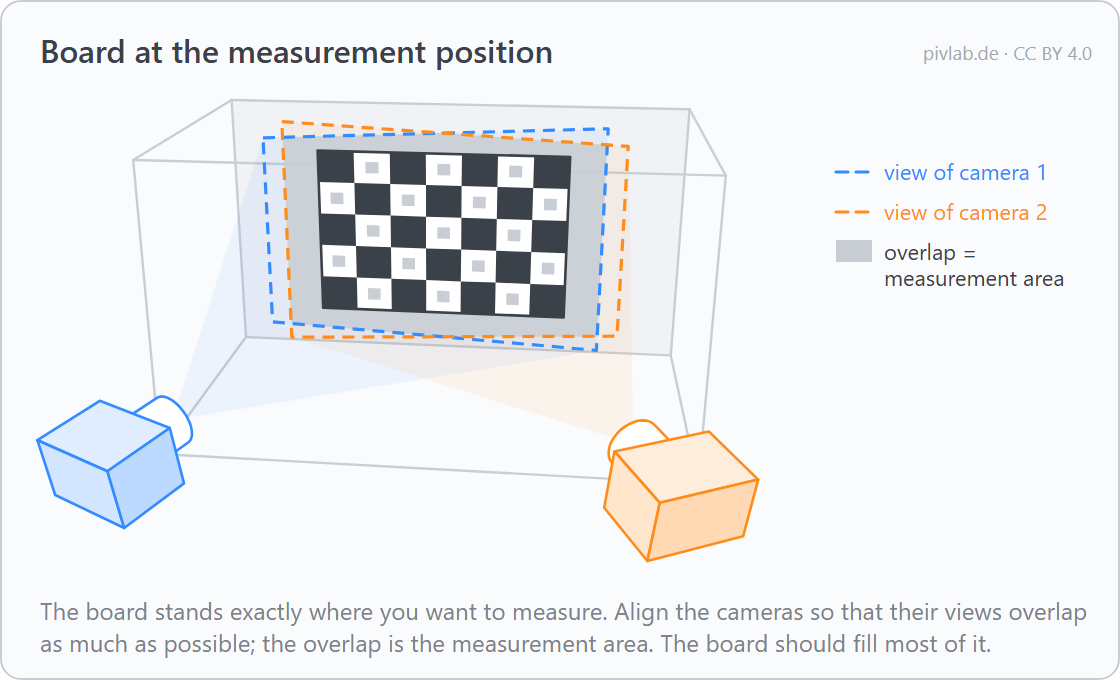
4. Board at the measurement position
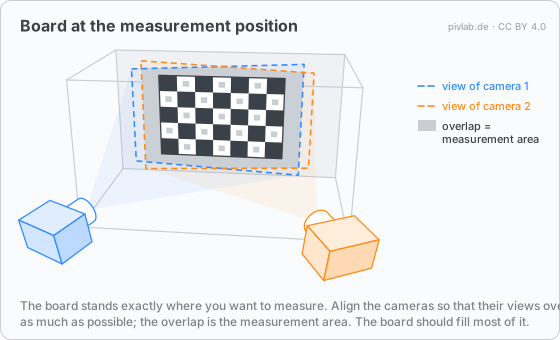
Put the board exactly where you want to measure: its surface defines the measurement plane. Both cameras must see it. Align the cameras so that their views overlap as much as possible; only the overlap can be measured with both cameras. The board should fill most of the overlap.
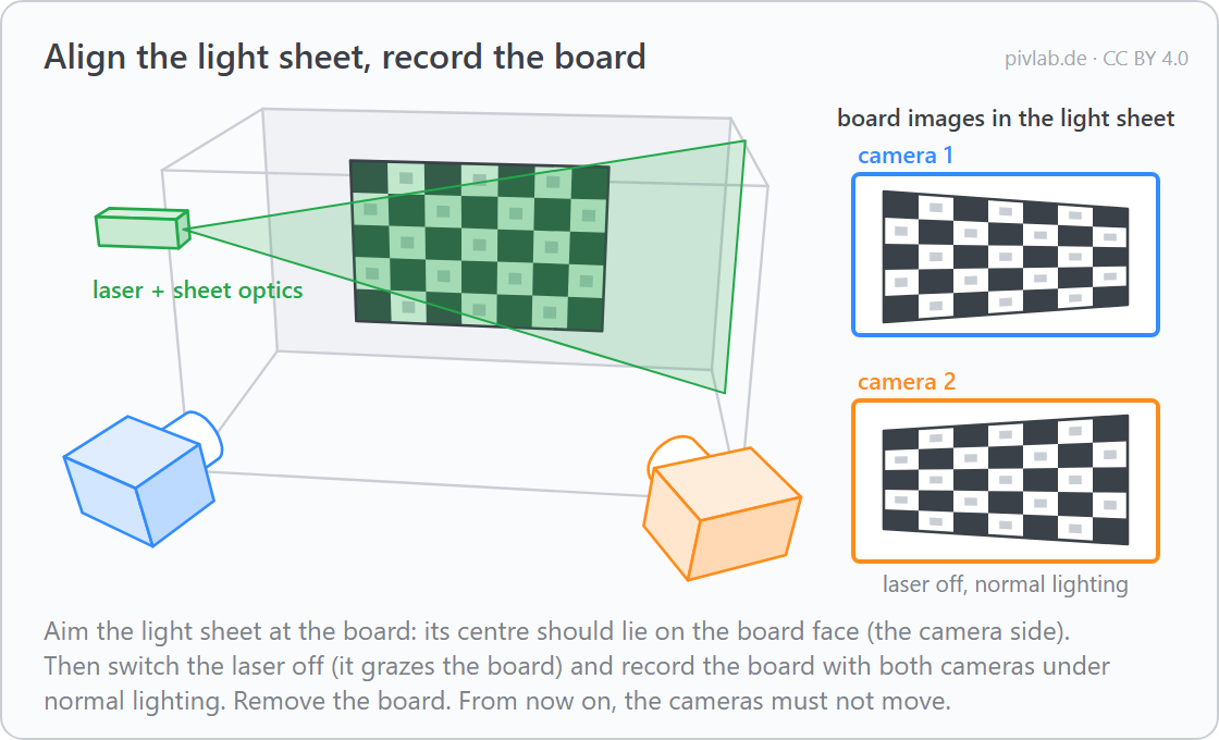
5. Align the light sheet, record the board
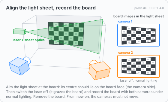
Switch the laser on and aim the light sheet at the board: the centre of the sheet should lie on the board surface that faces the cameras. Then switch the laser off – the sheet only grazes the board and lights it badly – and record the board with both cameras under normal lighting: these are the board images in the light sheet. Remove the board. From now on the cameras must not move. A small offset between sheet and board is not a problem; it is measured and corrected in step 7.
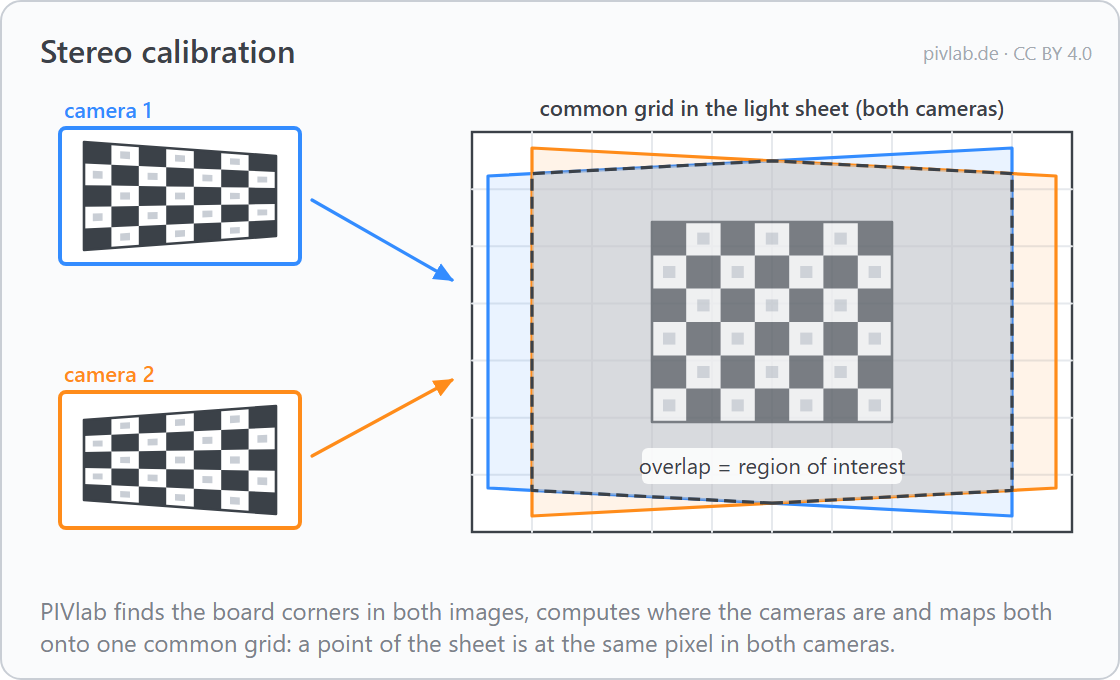
6. Stereo calibration
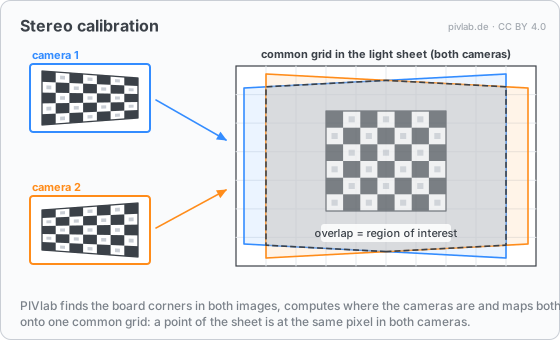
From the board corners in both board images, the stereo calibration computes where each camera is and how it looks at the board. Both camera images are then mapped onto one common grid in the plane of the light sheet: a point of the sheet lies at the same pixel in both cameras. The overlap of the two views becomes the region of interest, and the grid gives the scale (pixels to millimetres).
7. Record the flow, correct the disparity
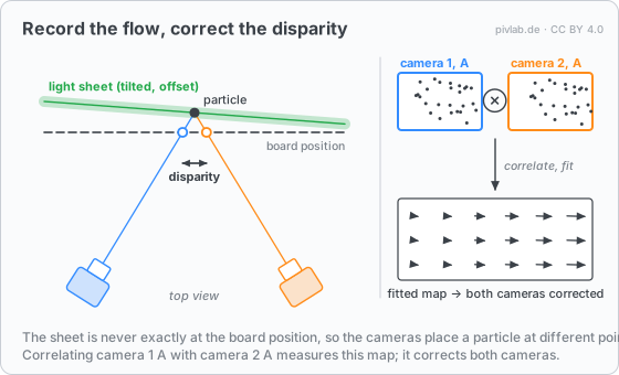
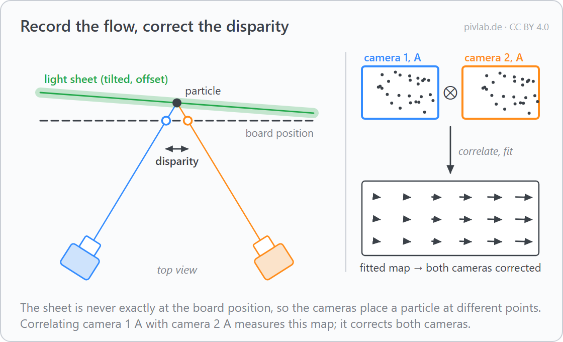
Now seed the flow and record image pairs with both cameras, synchronized with the laser. The board is never exactly at the position of the light sheet. The calibration places every particle on the board plane, so each camera puts the same particle at a slightly different point: the disparity. Correlating the particle images of camera 1 with those of camera 2 (recorded at the same moment) measures this shift everywhere in the image. A smooth map fitted to it corrects both cameras, and it also tells where the light sheet really is and how it is tilted. This step is often called self-calibration.
8. Analysis: from both cameras to u, v and w
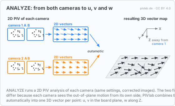
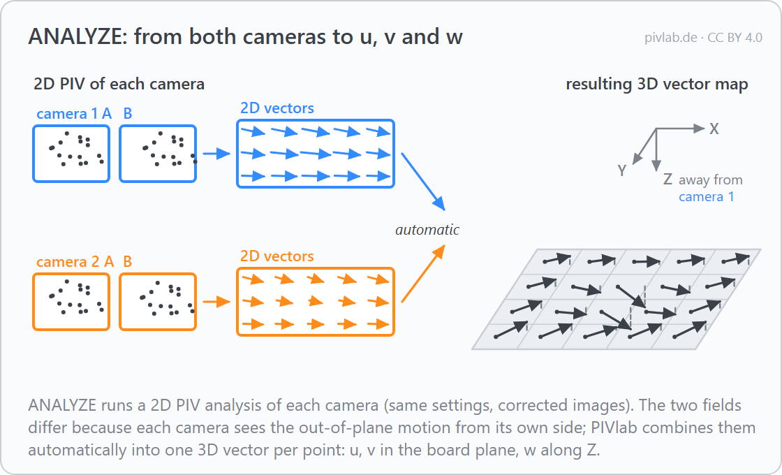
Each camera is analysed with normal 2D PIV, with the same settings and on the corrected images. The two 2D vector fields differ, because each camera sees the out-of-plane motion from its own side. For every point, the two measured 2D displacements (four numbers) are combined into one 3D vector: u and v in the board plane (X to the right, Y down in the image) and w along Z, away from camera 1. In PIVlab this combination happens automatically after the analysis, and again after each validation.
Use these drawings
The drawings may be used freely, e.g. in lectures, theses and presentations, under the licence CC BY 4.0. Please credit them as “Drawings: PIVlab, www.pivlab.de, CC BY 4.0”.
- Overview: SVG · PNG
- Step 1: SVG · PNG
- Step 2: SVG · PNG
- Step 3: SVG · PNG
- Step 4: SVG · PNG
- Step 5: SVG · PNG
- Step 6: SVG · PNG
- Step 7: SVG · PNG
- Step 8: SVG · PNG
Try the procedure without any hardware: PIVlab’s 3D flow and stereo-PIV simulator creates images of two virtual cameras, including calibration boards. How PIVlab records and analyses stereo-PIV: Stereo-PIV software and the manual pages Stereo-PIV: set-up and recording, Stereo acquisition and Stereo-PIV analysis.